10 Essential Google Sheets Functions for Marketers

As a marketer, your success depends on your ability to analyze data and derive insights that help you make data-driven decisions. However, with the vast amount of data at your disposal, it can be overwhelming to try and make sense of it all. That's where functions come in. Functions are a powerful tool that can help you organize, analyze, and extract information from your data with ease.
In this post, we'll explore the top 10 essential functions for marketers and practical examples to better understand their applications. Be sure to reference this spreadsheet I created while reading this blog post so you can follow along! These functions will not only make your job easier but also help you uncover insights that can drive your marketing strategy forward.
Let's dive in!
TL;DR
IF
SUMIFS
AVERAGEIFS
COUNTIFS
VLOOKUP
IFERROR
CONCATENATE
TRANSPOSE
TRIM
LEFT/RIGHT
1. IF
IF function is the fundamental of all. It’s a logical function that allows you to specify a condition and a result. If the condition is true, the function returns one result; if the condition is false, the function returns a different result. This can be useful for creating customized reports or analyzing data based on specific criteria.
=IF(logical_expression, [value_if_true], [value_if_false])
logical_expression: This is the condition that you want to test. If the condition is true, the function will return the value_if_true argument. If the condition is false, the function will return the value_if_false argument.
value_if_true (optional): This is the value that the function will return if the logical_expression is true. If you omit this argument, the function will return TRUE.
value_if_false (optional): This is the value that the function will return if the logical_expression is false. If you omit this argument, the function will return FALSE.
Having trouble following? Don’t forget to open the spreadsheet to follow along, if you haven’t already!
In the spreadsheet, we have a list of customer orders, including customer info like name, email, order date, and product name. Using these functions, we can analyze the data in various ways to gain insights and make informed marketing decisions.
In this first example, we want to know if customers are "active customers” or “inactive customers.” We can use the function:
=IF(D2 < TODAY()-90, "Inactive", "Active")
Essentially, we're checking the value in cell D2 (the date of the customer's last purchase) against the current date minus 90 days, i.e., whether the customer made a purchase in the last 90 days. If the value is less than that date, the function returns "Inactive"; otherwise, it returns "Active."
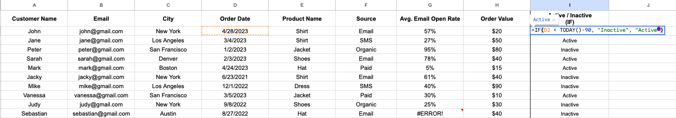
Sebastian is considered an “inactive customer” because his last purchase was more than 90 days ago.
2. SUMIFS
As a marketer, you may want to know which product contributed the most revenue. And what better way to do that than by adding up the numbers? That’s where SUMIFS comes in. It’s a function that adds up values based on multiple criteria.
=SUMIFS(sum_range, criteria_range1, criteria1, [criteria_range2, criteria2], ...)
sum_range: This is the range of cells that you want to sum based on the specified criteria.
criteria_range1: This is the range of cells that you want to apply the first criteria to.
criteria1: This is the first criterion that you want to apply to the criteria_range1.
criteria_range2, criteria2, ... (optional): These are additional ranges and criteria that you want to apply to the sum_range. You can include up to 127 additional criteria in this way.
For example, let’s say I want to find out how much revenue was generated from shirt orders in the last 60 days:
=SUMIFS(H:H, D:D, ">="&”4/30/2023”-60, D:D, "<="&”4/30/2023”, E:E, "Shirt")
You can also use the TODAY() function to get today's date, instead of "4/30/2023", so that the formula adjusts automatically. I use a fixed date above just for demonstration purposes.
=SUMIFS(H:H, D:D, ">="&TODAY()-60, D:D, "<="&TODAY(), E:E, "Shirt")

Shirts generated $70 over the past 60 days.
3. AVERAGEIFS
Instead of summing values, AVERAGEIFS calculates the average of values that meet specific criteria. This can be useful for analyzing data based on multiple factors.
=AVERAGEIFS(criteria_range1, criteria1, [criteria_range2, criteria2], ...)
criteria_range1: This is the range of cells that you want to apply the first criteria to.
criteria1: This is the first criterion that you want to apply to the criteria_range1.
criteria_range2, criteria2, ... (optional): These are additional ranges and criteria that you want to apply to the criteria_range1. You can include up to 127 additional criteria in this way.
For example, you could use the AVERAGEIFS function to calculate the Average Order Value (AOV) for customers in a specific city:
=AVERAGEIFS(B:B, C:C, "New York")

The Average Order Value for New York is $30.
4. COUNTIFS
Similar to SUMIFS and AVERAGIFS, COUNTIFS counts the number of cells that meet multiple criteria.
=COUNTIFS(criteria_range1, criteria1, [criteria_range2, criteria2], ...)
criteria_range1: This is the range of cells that you want to apply the first criteria to.
criteria1: This is the first criterion that you want to apply to the criteria_range1.
criteria_range2, criteria2, ... (optional): These are additional ranges and criteria that you want to apply to the criteria_range1. You can include up to 127 additional criteria in this way.
In the example below, we use the COUNTIFS function to count the number of shirt orders:
=COUNTIFS(E:E, "Shirt")

3 shirt orders were placed.
5. VLOOKUP
VLOOKUP searches for a value in the first column of a table and returns a corresponding value in the same row from another column in the table. This is particularly useful when you have a large data set and need to look up specific information.
=VLOOKUP(search_key, range, index, [is_sorted])
search_key: The value you want to look up in the first column of the range.
range: The range of cells that you want to search for the search_key. The range must include the column that contains the search_key and the column that contains the value that you want to return.
index: The number of the column in the range that contains the value that you want to return. The index is counted from the leftmost column in the range, with the leftmost column being 1.
is_sorted (optional): This is a logical value that specifies whether the range is sorted in ascending order. If is_sorted is TRUE or omitted, the range is assumed to be sorted in ascending order, and the function will use an approximate match to find the closest value that is less than or equal to the search_key. If is_sorted is FALSE, the function will use an exact match to find the exact value that matches the search_key.
In this example, we use VLOOKUP to retrieve each customer's Lifetime Value (LTV) from the separate LTV tab, based on their email addresses:
=VLOOKUP(B2, LTV!B:C, 2, FALSE)
The part “LTV!B:C” means it’s referencing columns B & C from the separate LTV tab in the sheet.


Grabbed LTVs from the separate LTV tab.
6. IFERROR
Have you ever encountered an error message in your spreadsheet and wished you could hide it? IFERROR is the function for you. It allows you to return a value if a formula results in an error, and a different value if the formula does not result in an error.
=IFERROR(value, value_if_error)
value: This is the cell that you want to test for errors. If it returns an error, i.e. “#ERROR!” the function will return the value_if_error argument instead.
value_if_error: This is the value that you want to return if the formula in the value argument returns an error.
Let’s say we have a formula that calculates the email open rate, but the formula results in an error. You can use IFERROR to show a message like “N/A” instead of the error message:
=IFERROR(G11, "N/A")

You can also set it to display “0%” as well, instead of “N/A”.
7. CONCATENATE
Concatenate combines two or more strings of text into one.
=CONCATENATE(text1, [text2], [text3], ...)
text1: This is the first text value that you want to combine.
text2, text3, ... (optional): These are additional text values that you want to combine. You can include up to 30 text values in this way.
Let’s say you want to send a personalized email to each customer thanking them for their recent purchase. You can use CONCATENATE to combine the customer’s name and product name with a pre-written message:
=CONCATENATE("Hey ", A2, ", Thank you for your recent purchase! ", " We hope you enjoy your ", lower(E2))
which creates the message “Hey John, Thank you for your recent purchase! We hope you enjoy your shirt”

8. Transpose
Transpose allows you to flip the orientation of data in a range of cells. This can be useful for reformatting data for different purposes, such as creating charts or graphs.
=TRANSPOSE(array)
array: This is the range of cells that you want to transpose. The TRANSPOSE function will switch the rows and columns of the array, so that the rows become columns and the columns become rows.
For example, you could use the Transpose function to flip the whole table from horizontal to vertical:
=TRANSPOSE(Main!A1:H11)
The result is in the “TRANSPOSE” tab in the sheet.

Columns and rows are flipped using TRANSPOSE.
9. TRIM
TRIM removes any leading or trailing spaces from a text string, but it leaves any spaces between words intact. It's useful when you want to clean up data and ensure that there are no extra spaces that could interfere with your calculations or analysis.
=TRIM(text)
text: This is the text string that you want to trim. Again, the function only removes any leading or trailing spaces from the text.
For example, we use TRIM to remove extra spaces at the beginning and end of " Email ". If you click cell F2, you will notice there are extra spaces. Here is the function:
=TRIM(F2)

10. LEFT/RIGHT
LEFT and RIGHT are functions that allow you to extract a certain number of characters from the beginning or end of a cell. This is useful when you need to extract specific information from a cell.
LEFT(text, [num_chars])
RIGHT(text, [num_chars])
text: This is the text string that you want to extract characters from.
num_chars (optional): This is the number of characters that you want to extract from the beginning of the text string. If you don't specify a value for this argument, the function will extract the first character only.
The LEFT function is used to extract a specified number of characters from the beginning of a text string in Google Sheets, whereas the RIGHT function is used to extract a specified number of characters from the end of a text string in Google Sheets.
Both the LEFT and RIGHT functions are useful for manipulating text strings in Google Sheets, such as extracting parts of a string, trimming excess characters, or concatenating multiple text strings together.
For example, let’s say you have a list of customer email addresses, but you only need the domain name. You can use the RIGHT function to extract the domain name from each email address:
=RIGHT(B2, LEN(B2) - FIND("@", B2))
This formula works by first finding the position of the "@" symbol in the email address using the FIND function. It then subtracts that position from the total length of the email address using the LEN, which gives you the number of characters in the domain name. Finally, it uses the RIGHT function to extract the specified number of characters from the end of the email address.

These are the top 10 essential functions! Google Sheets / Excel is a powerful tool that can make your life as a marketer easier. With these top 10 Google Sheet functions, you’ll be able to organize, analyze, and extract information from your data with ease.
Happy spreadsheet-ing!
Next Steps
Now that you've learned about these essential Google Sheet functions, it's time to put them into action!
Start by analyzing your marketing data using functions IF, SUMIFS, COUNTIFS, and AVERAGEIFS to gain insights into customer behavior and identify areas for improvement.
Use VLOOKUP, TRIM, and IFERROR to clean up your data and ensure accuracy, and CONCATENATE and TRANSPOSE to format and organize your data for easier analysis.
Finally, don't forget to use LEFT/RIGHT to extract and manipulate specific parts of your data for even deeper insights. With these powerful functions at your fingertips, you can take your marketing analysis to the next level!